
To gain insight into the behavior of our aircraft in flight, an aerodynamic model is necessary in lieu of a physical model from which wind tunnel data may be gathered. With a sufficiently accurate program, the wind tunnel data can be approximated to within the margin of error required for the effective design of a control system.
The program AVL was used to model the aircraft's behavior across a sweep of angles of attack. As AVL has been validated a number of times and is used in the development of aerodynamic models for popular commercial autopilot solutions, it was assumed to be sufficient for our current purposes. AVL models lifting surfaces with a vortex lattice method.
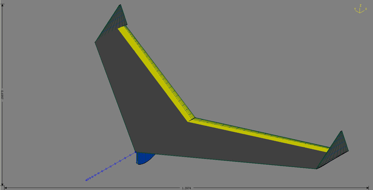
Shown is an image of the aircraft as modeled. The major features are captured by the model while things such as antenna, etc. which have no significant effect on the aerodynamics of the aircraft are ignored. It is likely that the pitot tube extending from the front of the aircraft could have been ignored as well, but it is included for completeness.
The designer's experience as well as basic aerodynamic knowledge are involved in the verification of the aerodynamic model. The resulting aerodynamic coefficients for a given trimmed airspeed are provided to the aircraft dynamics model for simulation purposes. What results is an aircraft model that does a reasonable job of approximating the actual behavior of the aircraft on which the simulation is based.
Dynamics Modeling:
With the aerodynamic data, a mathematical model of the dynamics and kinematics of the aircraft can be generated based on the laws of physics. The mathematical model will necessarily include approximations, however, it should model the aircraft "well enough" for our purposes. The dynamics model is used to save time by simulating the performance of the aircraft given a designed controller and the performance of that controller can be relatively easily analyzed.
The non-linear equations used in this mathematical model are well developed and can be found in several references. What results is a full six degree of freedom aircraft model.
Linearized Aircraft Model:
To use traditional control system design methods such as pole-placement, a linearized model of the system is required. Numerical linearization of the non-linear aircraft dynamics model is performed. Algebraic linearization of the aircraft model is possible, however, the assumptions typically tied in with this method are limiting. Algebraic linearization typically involves assuming the aircraft to be in non-accelerating, wings-level flight with small aerodynamic angles. Numerical linearization is better able to capture the aircraft dynamics in the absence of these assumptions, though the resulting state derivatives are only approximate.
Small perturbations in both the state and input from the trimmed flight condition are taken. Using Taylor series expansion, the first partial derivatives of the aircraft states with respect to these perturbations are obtained. The resulting linear time invariant state equations are taken to be the linearized aircraft model.
The linearization and simulation are performed in MATLAB, thus the round-off error is limited due to the double precision arithmetic inherent to the program. This is important because the perturbations used to develop the linear model can be very small. In a future implementation of a similar aircraft control system, the availability of the linear state matrices is powerful as it allows for more complex controllers that, with knowledge of the aircraft model, can predict the effect of a control input using tools such as a Kalman filter.
With the linearize state space equations, the actual controllers that will be detailed were designed initially using pole placement in MATLAB. This allowed for the performance of each controller to be adjusted such that the desired aircraft behavior could be tracked.
Separation of Lateral/Directional and Longitudinal Control:
The design of an aircraft controller is fortunately simplified by the fact that the longitudinal and lateral/directional dynamics of the aircraft can be largely separated in most flight modes. This means that a longitudinal controller, such as an airspeed tracking controller, may be designed independently of a bank-angle holding controller. The application of the longitudinal controller can then be assumed to have little effect of the performance of the lateral/directional controller.
Inner/Outer Loop Control:
The longitudinal controller for tracking airspeed is addressed first. The inner loop controller is wrapped around the aircraft pitch angle. The output of this controller is the required elevator deflection to hold the commanded pitch angle. The pitch-attitude hold control system is a typical inner loop control for most autopilots, but it is rarely used in isolation. In addition to helping track airspeed, this controller is able to damp out the short-period dynamics of the aircraft as well as increases the damping of the slower phugoid mode.
The outer loop longitudinal controller tracks a desired airspeed and results in a commanded pitch angle. The structure of this controller can frequently be much simpler, with a proportional gain usually sufficing to hold a desired airspeed. The structure of the designed longitudinal control system is similar to how a pilot controls airspeed in an aircraft, where pitch angle is used to control airspeed.
The designed controller is, in simulation, able to track a range of airspeeds from 8-15 meters per second. Additional care in the design of this control system should make it robust to more drastic airspeed changes.
The lateral/directional control implemented here commands an aircraft bank angle with aileron input. The inner loop closes a feedback loop around the roll-rate of the aircraft. This is because ailerons have direct control of aircraft roll rate and less direct control over the aircraft bank angle. The outer loop takes a commanded bank angle and returns a commanded roll rate when the loop is closed around bank angle. The primary implementation thus far has been to hold the aircraft wings level. As more complex missions evolve, the ability to hold a desired bank angle can be used as an inner loop controler for such things as a heading tracking controller or one that follows waypoints.
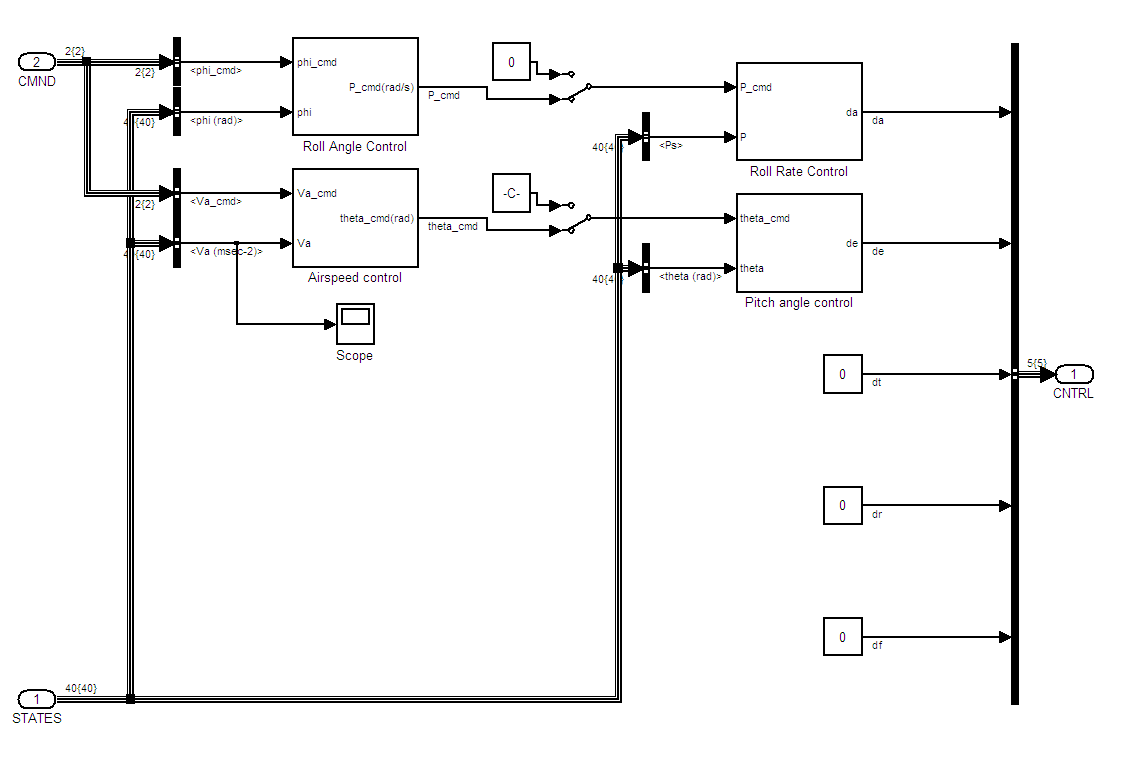
The aircraft controllers are implemented in Simulink such that their performance can be assessed. The Simulink model simulates the non-liner aircraft dynamics. The controller gains are further tuned at this step to achieved the desired aircraft performance. Simulink provides a powerful tool for rapidly prototyping the aircraft controllers.

Discrete Implementation:
A discrete version of a PID controller is used (though all of the gains, proportional, integral, and derivative are not always used). With the gains tuned in Simulink, the discrete controller is simply applied given the aircraft sets obtained in the other parts of this project.
The aircraft used in this experiment has only two control surfaces, one elevon on each wing. The implementation of the control system thus mixed aileron and elevator inputs on these surfaces. The elevator and aileron input commanded by the controllers are simply added to one another to produce the commanded actuation.